Virtualizing FPGAs in the Cloud
Authors: Yue Zha, Jing Li
Venue: ASPLOS 20
Institution: University of Pennsylvania
Point-Voxel CNN for Efficient 3D Deep Learning
Authors: Zhijian Liu*, Haotian Tang*, Yujun Lin, Song Han
Venue: NIPS 2019
Institution: MIT & SJTU
Background
- Voxel-based methods cannot scale to high resolution. Point-based methods have poor data locality (sparse data access).
Contribution
Point-Voxel CNN combines the best from both worlds
Point-Voxel Convolution: coarse voxelization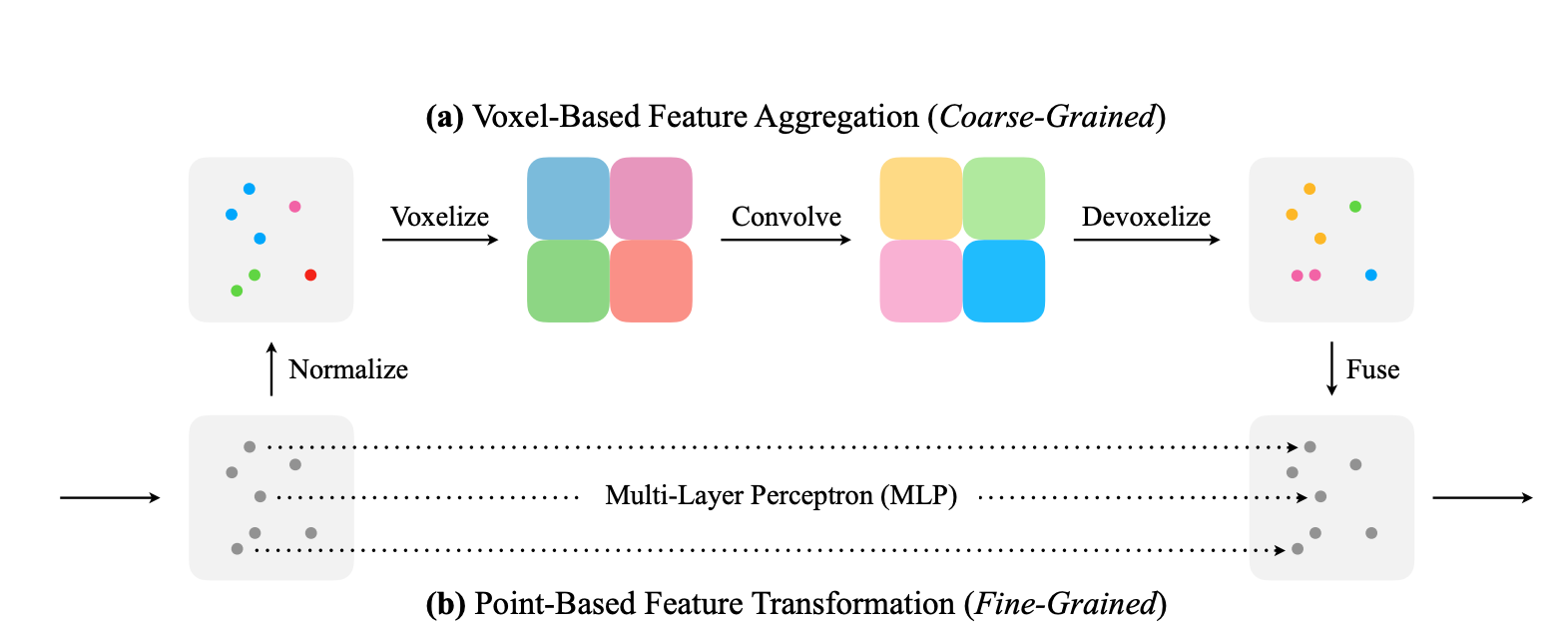
- Normalize: spatial locations (x,y,z) are normalized to [0,1] first.
- Voxelization: points that fall into the same voxel grid are averaged.
- Convolve: 3D convolution.
- Devoxelize: trilinear interpolation.
- Fuse: add interpolated point to MLP output points.
- PVCNN represents the input data as point cloud to reduce memory consumption. Voxel branch can be coarse as detail information is preserved with point branch.
- PVCNN leverages voxel-based convolution to obtain contiguous memory access pattern. No convolution with point-cloud, no dynamic-kernel and KNN computation, so random memory access is avoided.
Q&A
1. First of all, what is Voxel?
Voxel is like the 3D equivalence of pixel. A voxel represents a single sample, or data point, on a regularly spaced, three-dimensional grid.
2. What are voxelization and devoxelization?

3. What is Volumetric Convolution?
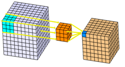
Section 3 gives a formal introduction of the volumetric convolution. We see that volumetric convolution is actually 3D convolution:
4. Why point-based methods have sparse data access?
- Neighbor points are not stored contiguously in the point representation so indexing them requrest a nearest neighbor search.
- Becasue relative positions of neighbors are not fixed, these point-based models have to generate the convolution kernels dynamically based on different offsets.
(Dynamic kernel is a special kind of method)
5. Why random memory access causes bank conflict?
[28] Onur Mutlu. DDR Access Illustration.
6. Why voxel-based method consumes more memory than point-cloud based method? Doesn’t it have less information because some of the points are merged into one voxel?
I’m not exactly sure about the answer right now. One guess is that during voxelization, the space where it doesn’t have any point is also voxelized. Maybe that’s why we could use sparse voxel.
Interesting Facts
- The computation cost and memory footprint of voxel-based models grow cubically with input resolution.
Searching Efficient 3D Architectures with Sparse Point-Voxel Convolution
Authors: Haotian Tang*, Zhijian Liu*, Shengyu Zhao, Yujun Lin, Ji Lin, Hanrui Wang, Song Han
Venue: ECCV 2020
Institution: MIT & Tsinghua University
Background
Previous models for 3D segmentation is still memory-intensive, so they can’t affort high resolution.
Small objects often become indistinguishable because of aggressive downsampling or coarse voxelization.
Contributions
A new 3D module: SPConv (Sparse Point-Voxel Convolution)
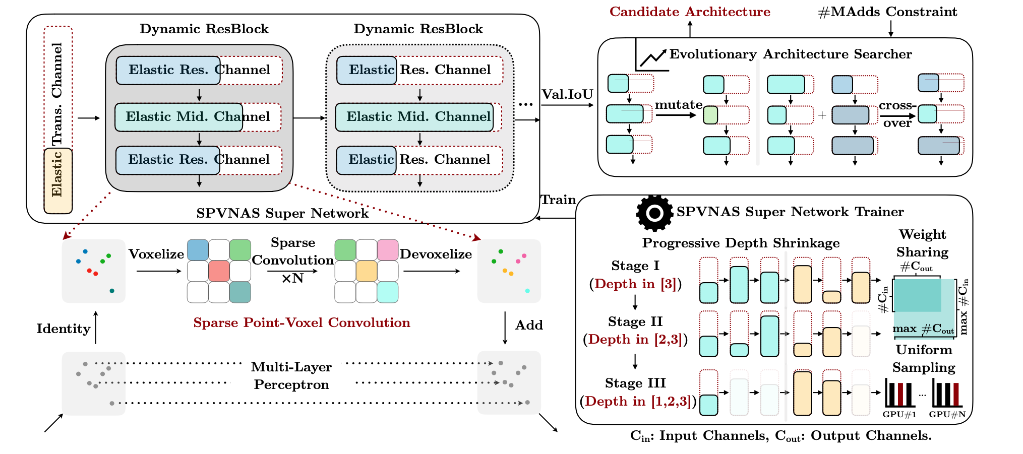
Input point-cloud is the same as before, but voxelization is sparse, i.e., it produces sparse voxel grid.
p.s. The author also talked about implementing sparse voxelization with GPU Hash table.Sparse convolution
From: Minkowski CNN: 4D Spatio-Temporal ConvNets.
“Sparse convolution” is actually a stack of sparse residual blocks.Devoxelization is the same: trilinear interpolation.
3D NAS with SPConv - SPVNAS
Design Space: fine-grained channel numbers, fixed kernel size.
The design space is very much like OFA - elastic channel numbers, elastic depth. It also uses progressive shrinking (depth) to train supernet. Differences are:- OFA has fixed input/output channel number for blocks, only the middle layer’s channel can change (by a expansion ratio). SPVNAS allows all channels to change.
- SPVNAS has a fixed 3x3x3 kernel size. This is because larger kernels are computationally expensive (cubic). Also sparse convolution brings significant overhead to build larger kernels.
Search method: single-objective Genetic Algorithm with MAC constraint. Candidates that don’t meet the constraint are discarded.
Q&A
1. Won’t sparse PVConv cause random memory access?
I suppose so. There must be random memory access while building the sparse kernel.
2. Elaborate on sparse conv?
From: Minkowski CNN: 4D Spatio-Temporal ConvNets.
Also: Sparse convolutional neural networks
Interesting Facts
- Point-based methods (point cloud and rasterized voxel grids) waste up to 90% of their time on structuring the irregular data.
Overwrite Quantization: Opportunistic Outlier Handling for Neural Network Accelerators
- Unpublished preprint
- Authors: Ritchie Zhao, Christopher De Sa, Zhiru Zhang
- ArXiv
TL;DR: A quantization scheme where the outlier could overwrite its neighbor value, and a low-overhead hardware implementation of the idea.
Basic Idea
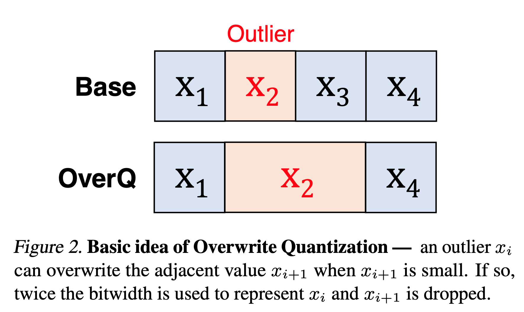
The basic idea of OverQ is to let outlier number take the bits of its neighbor to store its value.
OverQ is an opportunistic quantization scheme, meaning that $x_2$ will only overwrite $x_3$ only if $x_3$ is small. If $x_3$ is overwritten, its value is treated as zero. There are two types of OverQ: OverQ-Split and OverQ-Shift.
Two types of OverQ
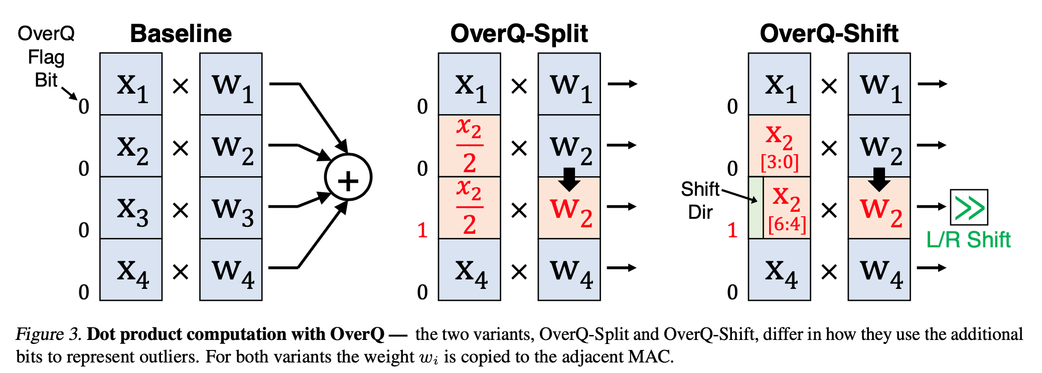
We take dot product of two vectors as an example. Both methods use a flag bit to indicated whether it is overwritten.
OverQ-Split
The outlier is divided by two to save in both positions. Then the weight is copied. The dynamic range is extended from $[0,2^n-1]$ to $[0, 2^{n+1}-1]$ for UInt.
OverQ-Shift
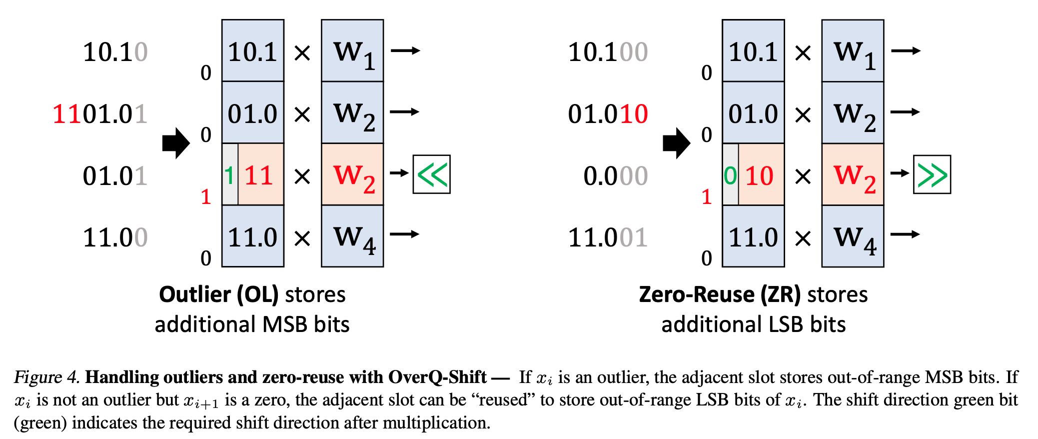
OverQ-Shift reserves one bit to indicate shift direction. Then the other bits can be used to store the extra LSB or MSB. This way it has $2 \times n - 1$ bits.
There is an extra mode called zero-reuse: when the neighbor is zero, it uses the extra bits to store LSB for higher precision. For example:
Q&A
1. Once you re-arrange the weight kernels, the output channels’ order is also going to change. Do we change them back? Or doesn’t it affect the convolution result in the downstream layer?
I was wondering if channel reordering would change the hardware design, and now I suppose it wouldn’t. My idea of implementing this: suppose we have two conv layers, first we permute the conv kernels in the first layer to get desired output channel order. Then we must permute the channel order of the second conv layer’s kernels accordingly. Then the hardware just runs the neural network as if it was never channel-reordered.
An overview of proxy-label approches for semi-supervised learning
- A blog post by Sebastian Ruder. link
While unsupervised learning is still elusive, researchers have made a lot of progress in semi-supervised learning. This post focuses on a particular promising category of semi-supervised learning methods that assign proxy labels to unlabelled data, which are used as targets for learning.
Proxy labels are generated by the model itself or variants of it without any additional supervision. These labels can be considered as noisy or weak.
There are three categories of proxy-label learning:
- Self-training: using a model’s own predictions as proxy labels.
- Multi-view learning: train models with different views of the data, then use its predictions as proxy label.
- Self-ensembling: ensembles variations of a model’s own predictions and uses these as feedback for learning.
Self-training
Self-training uses the confident predictions as labels. There’s a pre-set confidence threshold. In every iteration, the model is trained on the labelled dataset, then make predictions on unlabelled data. Those predictions with confidence score over the threshold will be added to the labelled dataset.
The downside of self-training is that the model cannot correct its own mistakes. This effect is exacerbated if the domain of the unlabelled data is different from the labelled data.
Multi-view training
Multi-view training train multiple models with different views of the data. These views differs in many ways, such as the feature they use, the model architectures, or different parts of the dataset.
- Co-training: trian two identical models on two parts of the dataset, confident predictions of one model is added to the other’s training set.
- Democratic Co-learning: train many different models on complete dataset, then use them to predict unlabelled data. If many models all make confident predictions on some data, it will be added to the training set.
- Tri-training with disagreement: three models selected with diversity are trained first in each iteration, and the unlabelled data which two models agree but one model disagrees is added to the training set.
- Asymmetric tri-training: test and unlabelled data is from different domain than labelled training data. To accommodate this change, one of the models is trained only on proxy labels and not on labelled data, and uses only this model to classify target domain examples at test time. Also three models share the same feature extractor.
- Multi-task tri-training: aims to relieve the training expense of tri-training. All models share parameters and trained with multi-task learning. To prevent mult-task tri-training reduced to self-training, we add an orthogonality constraint to the loss term to ensure the diversity of softmax layer’s input.
Self-ensembling
Like tri-training, self-ensembling methods also uses many variants of the model. But it does not require the diversity of the variants. Self-ensembling approaches mostly use a single model under different configurations.
- Ladder networks: this method aims to make the model robust to noise. For unlabelled data, it first makes a prediction as the label, then add noise to the same data, and train the model with the prediction on clean data.
- Virtual Adversarial Training: If perturbing the original sample is not possible or desired, we can instead add the worst possible perturbation to the example in the feature space. This make the input an adversarial example. But this method does not require label, unlike adversarial training. To do so, first, an image is taken and an adversarial variant of it is created such that the KL-divergence between the model output for the original image and the adversarial image is maximized.
- Pi model: ensembles the predicitons of one model under two different perturbation of the input data and two different dropout conditions.
- Temporal Ensembling: still one model architecture, but the model ensembles its prediction that is accumulated over timesteps (past predictions).
- Mean teacher: still one model, the alternative edition has averaged-over-training parameters.
Semi-supervised Learning in Computer Vision
- blog post by Amit Chaudhary: link
This post is a nice visualization of the previous post.
4D Spatio-Temporal ConvNets: Minkowski Convolutional Neural Network
- Venue: CVPR 2019
- Institution: Stanford University
- Authors: Christopher Choy, JunYoung Gwak, Silvio Savarese
COO-format Sparse Tensor
COO = Coordinate Format, also known as ‘ijv’ or ‘triplet’ format. Basically it uses three lists to store the sparse matrix: row, col, data. So data[i] is value at (row[i], col[i]).
Minkowski engine extends the coordinates with two entries: time step $t_i$, and batch index $b_i$. So the sparse tensor is stored like this:
$\mathbf{f_i}$ is the feature vector at the associated coordinate.
Generalized Sparse Convolution
For 3D space point-cloud data, the coordinates are no longer integers, and for 3D convolution, the kernel tensor’s shape may not be cubic. So we need a sparse convolution algorithm that is generalized for any kernel shape, any coordinates:
- $u$: D-dimensional coordinate
- $\mathcal{N}^D$ is a set of offsets that define the shape of a kernel
- $\mathcal{N}^D (u, \mathcal{C}^{in})$ is the set of offsets from the center $u$, that exists in $\mathcal{C}^{in}$
- $\mathcal{C}^{in}$ (input coordinate) is not necessarily identical to $\mathcal{C}^{out}$ (output coordinate).
AXI HyperConnect: A Predictable, Hypervisor-levelk Interconnect for Hardware Accelerators in FPGA SoC
- Venue: DAC 2020
- Institution: Department of Excellence in Robotics & AI, Acuola Superiore Sant’Anna, Pisa, Italy
- Authors: Francesco Restuccia, et al.
In this work, a new hypervisor-level hardware component named AXI HyperConnect is proposed. It allows interconnecting hardware accelerators to the same bus while ensuring isolation and predictability.
Background

- PS (Processing System) includes one or more processors.
- PS and FPGA access a DRAM contoller to reach a shared DRAM memory.
- The AXI standard is simultaneous, bidirectional data exchange standard.
The integration phase of Hyperconnect
We assume that the IP description is provided in an XML format such as the popular IP-XACT. Each hardware accelerator should implement an interface composed of an AXI control slave interface and an AXI master interface.
- Each AXI master port of hardware accelerator is connected to an input slave port of an AXI HyperConnect.
- The master port of the AXI HyperConnect is connected to the FPGA-PS interface, while the hardware accelerator’s AXI slave ports are connected to the PS-FPGA interface.
- Once all accelerators have been connected, the system integrator uses a synthesis tool (Vivado, Quartus) to synthesize the overall design.
- Finally the bitstream is generated.
AXI HyperConnect Details
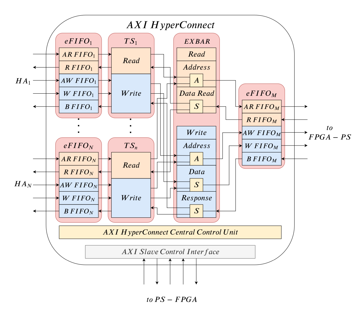
eFIFO (efficient FIFO)
The eFIFO module is a buffered AXI interface. Each eFIFO module defines five independent FIFO queues, one for each AXI channel. Each of the queues is implemented as a proactive circular buffer (proactive means always ready to receive).
decoupling mechanism: when a hardware accelerator is decoupled, the AXI handshake signals on all the AXI channels are kept low, not allowing data exchange.
TS (Transaction Supervisor)
TS is the core module to control bandwidth and memory access management. TS implementation detials: “Is your bus arbiter really fair?”. TS does the following things:
- splits read/write requests into sub-requests with nominal burst size and merges incoming data/write responses.
- A reservation mechanism: reserve a configurable budget of transaction for each input port that is periodically recharged (Time Division).
EXBAR (Efficient Cross-bar)
The EXBAR is a low-latency crossbar in charge of solving the conflicts of read/write requests. It implements round-robin artbitration with a fixed granularity of one trasaction per TS module in each round-cycle (thus the latency is predictable).
Cross-Modal Generalization: Learning in Low Resource Modalities via Meta-Alignment
- Venue: preprint for now
- Institution: CMU, University of Tokyo
- Authors: Paul Pu Liang, Peter Wu, Liu Ziyin, Louis-Philippe Morency, Ruslan Salakhutdinov
Overview
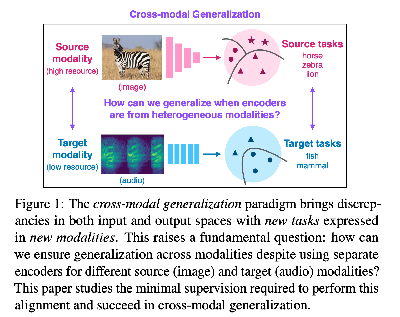
Modality
Input spaces, the means that a concept is expressed, or a type of representation. e.g.: visual, acoustic, tactile, ligustic are different modalities.
Key Research Question
- How to generalize across modalities when using seperate encoders for source and target modalities?
This problem statement differs from conventional meta-learning and domain adaptation in that the source and target modality do not share the same encoder. - What is the minimal extra supervision required to learn new output concepts expressed in new input modalities?
Goal/Motivation
To train models in high-resource source modality, and generalize models in low-resource (few labeled samples) target modality.
Key Concepts
Cross-modal generalization
A learning paradim to train a model that can
(1) quickly perform new tasks in target modality
(2) doing so while being trained on a different source modality
DADA: Differentiable Automatic Data Augmentation
- Venue: ECCV 2020
- Intitution: Peking University, Anyvision, Queesn University of Belfast, The University of Edinburgh
- Authors: Yonggang Li, Guosheng Hu, Yongtao Wang, Timothy Hospedales, Neil M. Robertson, Yongxin Yang
Related works
AutoAugment
AutoAugment is the pioneering work for automatic data argumentation. It uses Reinforcement Learning to solve an optimization problem: to maximze accuracy on validation dataset with selected augmentation scheme. It models the policy search problem as a sequence prediction problem, and uses an RNN controller to predict the policy. RL optimizes the controller parameters. Two parameters are optimized: the type of data augmentation, and the intensity of selected augmentation. AutoAugment is effective but very computationally expensive, searching augmentation scheme for single task on single dataset costs up to 5k GPU hours.Population Based Augmentation (PBA)
PBA introduces efficient population based optimization, which was originally used in HPO (Hyperparameter Opimization). Note: probabily evolutionary strategy.Fast AutoAugment (Fast AA)
Fast AA and PBA are both proposed to solve the efficiency problem of AutoAugment. Fast AA models the augmentation selection problem as a density matching problem, and solve it through Bayesian Optimization.
